Using the R Package Profvis on a Linear Model

Not all data scientists were computer scientists who discovered their exceptional data literacy skills. They come from all walks of life, and sometimes that can mean optimizing for data structures and performance isn’t the top priority. That’s perfectly fine! There may come a time where you find yourself executing a chunk of code and consciously noting you could go take a short nap, and that’s where you’ve wondered where you could to be more productive. This short example provides help in how to profile using an extremely powerful and user-friendly package, profvis.

Data for this example: https://data.detroitmi.gov/Public-Health/Restaurant-Inspections-All-Inspections/kpnp-cx36

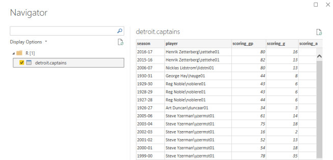
In this tutorial, we’ll create and profile a simple classifier. The dataset linked to above provides all restaurant inspection data for the city of Detroit, from August 2016 to January 2019.

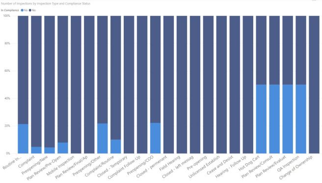
After extensive analysis and exploration in Power BI, some patterns emerge. Quarter 3 is the busiest for inspections, and Quarter 1 is the slowest. Routine inspections occur primarily on Tuesday, Wednesday, or Thursday. Hot dog carts are a roll of the dice.

Inspections by Quarter

Routine inspections by weekday

Inspections by Type

This doesn’t seem too complex, and we theorize that we can create a classifier that predicts whether a restaurant is in compliance, by taking into account the number of violations in each of three categories (priority, core, and foundation).

To do so, we throw together some simple code that ingests the data, splits into a test and training set, creates the classifier model, and provides us the confusion matrix.

# Import the restaurant inspection dataset
df.rst.insp <- read.csv("Restaurant_Inspections_-_All_Inspections.csv", header = TRUE)

# A count of rows in the dataset
num.rows <- nrow(df.rst.insp)

# Create a shuffled subset of rows
subset.sample <- sample(num.rows, floor(num.rows*.75))

# Create a training dataset using a shuffled subset of rows
df.training <- df.rst.insp[subset.sample,]

# Create a test dataset of all rows NOT in the training dataset
df.test <- df.rst.insp[-subset.sample,]

# Create the generalized linear model using the training data frame
mdlCompliance <- glm(In.Compliance ~ Core.Violations + Priority.Violations + Foundation.Violations, family = binomial, data = df.training)

# Predict the compliance of the test dataset
results <- predict(mdlCompliance, newdata=df.test, type = "response")

# Turn the response predictions into a binary yes or no
results <- ifelse(results < 0.5, "No", "Yes")

# Add the results as a new column to the data frame with the actual results
df.test$results <- results

# Output the confusion matrix
table(df.test$In.Compliance, df.test$results)

# Output the confusion matrix
library(caret)
confMat <- table(df.test$In.Compliance, df.test$results)
confusionMatrix(confMat, positive = "Yes")

An accuracy rate of 81.5%! That’s pretty great! Admittedly, a human wouldn’t have much trouble seeing a slew of priority violations and predicting a restaurant shutdown, but this classifier can perform the analysis at a much faster rate.

At this point, we have a good model we trust and expect to use for many years. Let’s pretend to fast forward a decade. Detroit’s meteoric rise has continued, the dataset has grown to massive amounts, and we begin to think we could improve the runtime. Easy enough! Profvis is here to give us the most user-friendly introduction to profiling available. To begin, simply install and load the package.

install.packages("profvis")
library("profvis")

Wrap your code in a profvis call, placing all code inside of braces. The braces are important, and be sure to put every line you want to profile. Maybe your confusion matrix is the bad part, or maybe you read the CSV in an inefficient way!

profvis({

df.rst.insp <- read.csv("Restaurant_Inspections_-_All_Inspections.csv", header = TRUE)
num.rows <- nrow(df.rst.insp)
subset.sample <- sample(num.rows, floor(num.rows*.75))
df.training <- df.rst.insp[subset.sample,]
df.test <- df.rst.insp[-subset.sample,]
mdlCompliance <- glm(In.Compliance ~ Core.Violations + Priority.Violations + Foundation.Violations, family = binomial, data = df.training)
results <- predict(mdlCompliance, newdata=df.test, type = "response")
results <- ifelse(results < 0.5, "No", "Yes")
df.test$results <- results
confMat <- table(df.test$In.Compliance, df.test$results)
confusionMatrix(confMat, positive = "Yes")

})

The output can help pinpoint poor-performing sections, and you can appropriately improve code where necessary.

The FlameGraph tab gives us a high-info breakdown. The Data tab gives us the bare-bones stats we need to get started.

profvis FlameGraph

profvis Data tab

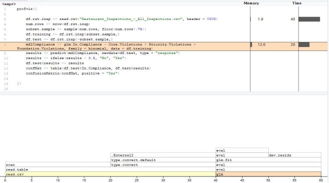
In this example, we would certainly choose to improve the way we read in the data, since it accounts for two-thirds of the total run time in that single step!

The result here might be a minor gain, but we can easily understand how larger datasets would see massive performance improvements with a series of tweaks.


When to Use M or R in Power BI

Recently, I was working on a large assignment involving complex data manipulation inside Power BI when a co-worker asked me a question I’m no stranger to: “Why are you doing that in M? Why not use R?”

I stammered through a few reasons until they felt comfortable, but ultimately left with the question still in my mind. I wanted a more crisp and clear answer. This post should hopefully clear up some understanding or misconceptions on how each works within Power BI, and some strengths or weaknesses. Keep in mind, this never has to be either-or! M can easily come without R, but R will almost never come in Power BI without M.

A Couple General Rules

Use what you’re comfortable with

These aren’t one-size-fits-all answers. Your situation will vary, and it’s important to take your context into account when making a decision. Learning a whole new language is rarely the answer to a single problem you’ve encountered.

The cost of re-platforming

As a rebuttal to the item immediately above, when you’re handed a chunk of custom M or custom R, it’s natural to want to switch to what you’re comfortable with, but you should consider what this means. Introducing language complexities to an enterprise strapped for skilled resources can make a problem exponentially worse in the long-run. Know what your company uses, what your co-workers have, and what makes the most sense in your ecosystem. Convincing a bureaucratic organization to install R on a fleet of computers can be an overwhelming challenge, for example.

When to Use M

You’re distributing the PBIX file

I’m not here to admonish you for your blasé attitude toward version control! Maybe your organization doesn’t have Power BI Premium, but relies on Power BI for its reporting. Maybe you distribute files that rely on certain custom parameters so each person can see their own data. There are plenty of reasons why organizations choose to share PBIX files. When doing this, custom M code is generally preferable, because it’s all built into Power BI. A file using R requires each individual have R installed, all the same packages you’ve used, and preferably the same versions, to avoid package conflicts.

The dataset is larger than your computer’s memory

Remember that R stores its data in memory (unless you’re using RevoScaleR, but we can talk about that later!). Power BI Premium as of this article supports up to a 10GB dataset. If your enterprise uses 8GB or 4GB computers, you’re best sticking to M. Another tip for this situation is to create a VM in Azure with higher specs, dedicated to your Power BI development.

You want to protect the code, or consider it proprietary

Writing your own custom M connectors is a beautiful thing. This is the subject of an upcoming article more in-depth, but suffice it to say, if you’re using standard connections such as an Odata Service, XML, Web, or any others, and you consider the way you’re connecting to retrieve and manipulate the data to be proprietary to your company or you want to protect it from tinkering by users, you can package up all your M as a connector and use that alone. Note that this is a double edged sword – you need to distribute your connector to any users of the PBIX file, and keep it up to date!

Auditing code step-by-step will be necessary

Since Power BI writes its own M code as you clean and prep the dataset, this is a no-brainer. If you need to see what happened in each step along the way, it’s best to keep it all in M. You can absolutely do this using R, but each step will have to be its own separate code chunk, and you likely lose the data type of each column every time you run a new R script.

When to Use R

You need to unlock the power of custom visualizations

To be clear, this wouldn’t take the place of M! If you’re ever extremely picky about a tertiary axis, a hexbin map, a network diagram, or just need total control over what to display (hey, I get it, some clients have a vision and won’t budge), then writing it up in R is the best place to go. At this point, you’ve already introduced R to the solution, so feel more at ease introducing it in the data manipulation steps as well.

There are complex data structures to handle

Sometimes, you encounter a JSON or XML structure that really makes you scratch your head. “Who wrote this spec? What were they thinking? Were they thinking at all?” (In all fairness, each of us works under constraints that may not be immediately visible to others!) During this situation, I’ve found myself transposing tables, converting records to tables, taking each field to a new record, running 8 nested List.Transform’s, and… you get the picture. R, with the power of lapply and more, can often get the job done simpler and easier.

Multiple distinct data sources need to be ingested in one query

This is almost a corollary to the above point. If you’re connecting to multiple non-standard places, chances are there’s already an R package for it, and you’re best off pulling them all in, joining the data (shout-out to dplyr), and then creating the output set.

Sentiment Analysis in Power BI with Microsoft Cognitive Services

Today, we’re going to combine 2 powerful Microsoft tools into one analysis: Cognitive Services, and Power BI.

If you’re like me, you’re already doing your data analysis in Power BI. Similarly, you’re using Cognitive Services as your artificial intelligence multi-tool. But somehow, there isn’t a button in Power BI to “retrieve sentiment” for text, to “detect objects in image,” or to “extract key phrases” from a sentence. That’s alright. We’ll do the first one ourselves.

We’re going to kick this off assuming you already have Text Analytics endpoint and API Key. You’ll need the region from your endpoint, and the hexadecimal string that is the API key.

I’ve previously written and annotated code that allows any R programmer to use the Key Phrase and the Sentiment endpoint of the Text Analytics API. They full code is available in my GitHub repo, and will comprise most of the magic taking place.

You’ll need an interesting article to analyze. This works best for large text datasets from your customers, to help you build understanding of their underlying emotions without requiring you to read each one independently and understand the text. However, in this example, I’m parsing an opinion article from the Detroit Free Press about the Freedom of Information Act. It won’t make a difference; the steps are identical no matter your source.

First, load your dataset in. It should have 1 sentence per line from the article. If managing multiple data source, you may want to add extra metadata to identify different customers, different articles or sources, and other key information relevant to understanding the text.

Sentences

Once this is in, edit your query by choosing to add an R script

Run-R-Script

We’ll start by entering the full set of R scripts into the box. It loads our libraries (httr and rjson) and creates our functions.

# Extract key phrases uses Microsoft Cognitive Services API for Key Phrase

library(httr)
library(rjson)


cogAuth <- function(key) {

# Access key assignment for use in REST calls
 assign("keyCogServices", key, envir = envCogServices)

}

# Create the empty environment to store the key
envCogServices <- new.env(parent = emptyenv())


# Function for using Cognitive Services API
# Note: Can ONLY be used with keyPhrases OR sentiment
fnCogServicesBatch <- function(text.inputs, phrase.language = "en", endpoint = "keyPhrases", region = "eastus") {

# Coerce to character
 text.inputs <- as.character(text.inputs)

# The URL for Key Phrases cognitive service
 url.cog.service <- paste("https://", region, ".api.cognitive.microsoft.com/text/analytics/v2.0/", endpoint, sep = "")

# Create empty list in proper structure for request
 list.docs <- list(documents = list(list()))
 num.max <- length(text.inputs)

# For loop (unfortunately); 
 for (i in 1:num.max) {
 list.docs$documents[[i]] <- list(language = phrase.language, id = i, text = text.inputs[i])
 }

# Convert the list to JSON for posting
 json.body <- toJSON(list.docs)

# Post the call to the REST API
 raw.response <- POST(url.cog.service, add_headers(.headers = c("Ocp-Apim-Subscription-Key" = envCogServices$keyCogServices, "Content-Type" = "application/json")), body = json.body)

# Read in the response as character
 json.response <- readBin(raw.response$content, "character")

# Convert the character, now JSON, response back to a list
 list.response <- fromJSON(json.response)

# Extract the first element of each of these
 list.phrases <- lapply(list.response$documents, "[[", 1)

# Unlist to flatten all topics (does this break with score?)
 vec.words <- unlist(list.phrases)

# Important!
 tolower(vec.words)

}

For the calls to work, we have to do two things: Store our API key, and set the right configurations for region, language, and endpoint. My work is in the English language, the East US 2 region, and the Sentiment endpoint.

Set your API key by using the helper function cogAuth:

cogAuth("Your API key here!")

Then, after identifying which column has your records, coerce to a Character type. In my experience, this reduces the chances of odd behavior.

dataset$sentences <- as.character(dataset$sentences)

The nice part of my function is that it happily manages batch inputs. We’ll take advantage of that ability by throwing the entire column at the API, and assigning the return scores to a new column called ‘sentiment.’ This is also where we set the region, language, and endpoint!

dataset$sentiment <- fnCogServicesBatch(dataset$sentences, phrase.language = "en", endpoint = "sentiment", region = "eastus2")

As with any R scripts,  we’ll change the dataset to ‘output’ so Power BI identifies the resulting data we want to keep.

output <- dataset

Warning! You may run into an error like the one below for privacy levels. If so, please reference the official Microsoft documentation.

privacy

The output may generate as a table, as well. This is okay! Expand the column and bring all values with it.

output-table

Finally, we see our sentiment in one place.

Sentiments

Remember that the way sentiment is delivered, a 0 is “Extremely negative,” while a 0.5 is “Neutral” and 1.0 is “Extremely positive.” You may want to create a calculated column that subtracts 0.5 from all scores to give yourself a positive/negative view.


score

Congratulations! You’ve put two of Microsoft’s most powerful tools together to further your analysis. From here, your real work begins.

Score-by-index

Retrieve data.world data sets in Power BI using R

[update: the data.world connector is now available in beta, as a preview feature in Power BI. However, this post is relevant in case you’d like to manage what you retrieve through your own code]

data.world is a website promising “open, secure, social, and linked” data sets. Using external data sets is a great way to learn, benchmark against competition or industry, and spark new ideas. With this tutorial, we’ll show you how to use their R Library in Power BI to retrieve and build a simple visual of some basic information.

To begin, you’ll want to install their R SDK. The short version here is to open your favorite R IDE, and enter:

install.packages("data.world")

After, get your API key from data.world by going to advanced settings in your data.world profile. Open your favorite IDE back up, and make sure to save the API key so the library will have it on open in the future:

api_key_config <- data.world::save_config("API KEY")
data.world::set_config(api_key_config)

Find your favorite data set, and we can begin. For this exercise, I’ll choose the Original Six Hockey data set.

The author of this set is scuttlemonkey, the name is original-six-hockey, and the CSV I want in particular is DET-captains, a list of all captains of the Detroit Red Wings. This gives us everything we need.

In Power BI, choose ‘Get Data’ and then find ‘R Script’

RScript

Enter the following code into the window:

library(data.world)
detroit.captains <- query(qry_sql("SELECT * FROM `DET-captains`"), dataset = "scuttlemonkey/original-six-hockey")

Hit submit, and in no time, you’ll see a preview of a data frame containing all the Detroit Red Wings captains in their history!

DataFrame

From here, we have a dataset available for us to analyze in whatever ways we need within Power BI.

Total points in a season by each Detroit Red Wings captain from 1980 to 2017

With a data set analyzed, we can ask questions like:

What happened in the 2004-2005 season? (There was an NHL lockout)

Why are there two captains in 1980? (Reed Larson and Errol Thompson split captainship that season, with Errol Thompson eventually being traded to the Pittsburgh Penguins)