When to Use M or R in Power BI

Recently, I was working on a large assignment involving complex data manipulation inside Power BI when a co-worker asked me a question I’m no stranger to: “Why are you doing that in M? Why not use R?”

I stammered through a few reasons until they felt comfortable, but ultimately left with the question still in my mind. I wanted a more crisp and clear answer. This post should hopefully clear up some understanding or misconceptions on how each works within Power BI, and some strengths or weaknesses. Keep in mind, this never has to be either-or! M can easily come without R, but R will almost never come in Power BI without M.

A Couple General Rules

Use what you’re comfortable with

These aren’t one-size-fits-all answers. Your situation will vary, and it’s important to take your context into account when making a decision. Learning a whole new language is rarely the answer to a single problem you’ve encountered.

The cost of re-platforming

As a rebuttal to the item immediately above, when you’re handed a chunk of custom M or custom R, it’s natural to want to switch to what you’re comfortable with, but you should consider what this means. Introducing language complexities to an enterprise strapped for skilled resources can make a problem exponentially worse in the long-run. Know what your company uses, what your co-workers have, and what makes the most sense in your ecosystem. Convincing a bureaucratic organization to install R on a fleet of computers can be an overwhelming challenge, for example.

When to Use M

You’re distributing the PBIX file

I’m not here to admonish you for your blasé attitude toward version control! Maybe your organization doesn’t have Power BI Premium, but relies on Power BI for its reporting. Maybe you distribute files that rely on certain custom parameters so each person can see their own data. There are plenty of reasons why organizations choose to share PBIX files. When doing this, custom M code is generally preferable, because it’s all built into Power BI. A file using R requires each individual have R installed, all the same packages you’ve used, and preferably the same versions, to avoid package conflicts.

The dataset is larger than your computer’s memory

Remember that R stores its data in memory (unless you’re using RevoScaleR, but we can talk about that later!). Power BI Premium as of this article supports up to a 10GB dataset. If your enterprise uses 8GB or 4GB computers, you’re best sticking to M. Another tip for this situation is to create a VM in Azure with higher specs, dedicated to your Power BI development.

You want to protect the code, or consider it proprietary

Writing your own custom M connectors is a beautiful thing. This is the subject of an upcoming article more in-depth, but suffice it to say, if you’re using standard connections such as an Odata Service, XML, Web, or any others, and you consider the way you’re connecting to retrieve and manipulate the data to be proprietary to your company or you want to protect it from tinkering by users, you can package up all your M as a connector and use that alone. Note that this is a double edged sword – you need to distribute your connector to any users of the PBIX file, and keep it up to date!

Auditing code step-by-step will be necessary

Since Power BI writes its own M code as you clean and prep the dataset, this is a no-brainer. If you need to see what happened in each step along the way, it’s best to keep it all in M. You can absolutely do this using R, but each step will have to be its own separate code chunk, and you likely lose the data type of each column every time you run a new R script.

When to Use R

You need to unlock the power of custom visualizations

To be clear, this wouldn’t take the place of M! If you’re ever extremely picky about a tertiary axis, a hexbin map, a network diagram, or just need total control over what to display (hey, I get it, some clients have a vision and won’t budge), then writing it up in R is the best place to go. At this point, you’ve already introduced R to the solution, so feel more at ease introducing it in the data manipulation steps as well.

There are complex data structures to handle

Sometimes, you encounter a JSON or XML structure that really makes you scratch your head. “Who wrote this spec? What were they thinking? Were they thinking at all?” (In all fairness, each of us works under constraints that may not be immediately visible to others!) During this situation, I’ve found myself transposing tables, converting records to tables, taking each field to a new record, running 8 nested List.Transform’s, and… you get the picture. R, with the power of lapply and more, can often get the job done simpler and easier.

Multiple distinct data sources need to be ingested in one query

This is almost a corollary to the above point. If you’re connecting to multiple non-standard places, chances are there’s already an R package for it, and you’re best off pulling them all in, joining the data (shout-out to dplyr), and then creating the output set.

4 for 4.0.0 – Four Useful New Features in R 4.0.0

With the release of R 4.0.0 upon us, let’s take a moment to understand a few parts of the release that are worth knowing about.

list2DF Function

This is a new utility that will convert your lists to a data frame. It’s very friendly, in the sense that it attempts to avoid errors by making assumptions on how to fill in gaps. That could lead to heartache when those don’t align with what you’re expecting, so be careful!

> one <- list(1:3, letters[5:10], rep(10,7))
> list2DF(one)
        
1 1 e 10
2 2 f 10
3 3 g 10
4 1 h 10
5 2 i 10
6 3 j 10
7 1 e 10

sort.list for non-atomic objects

Vectors and matrices are the most common non-atomic objects in R. The function sort.list now works with these. Previously you could use order on either of these, but if you’ve chosen to employ sort.list within your functions, you won’t have to error handle the outcomes of non-atomic objects.

> mtx.test <- matrix(1:9, nrow = 3, byrow = TRUE)
> sort.list(mtx.test)
[1] 1 4 7 2 5 8 3 6 9


New Color Palettes!

You can check out the new palettes using the palette.pals function. R has always been strong in visualizations, and while Detroit Data Lab won’t endorse Tableau color schemes, we’re excited to see the better accessibility offered by some color palettes. See the new R4 palette below using a simple code snippet.

> palette("R4")
> palette()
[1] "black"   "#DF536B" "#61D04F" "#2297E6" "#28E2E5" "#CD0BBC" "#F5C710" "gray62" 
> show_col(palette())

R version 4.0.0 color palette

stringsAsFactors = FALSE

You knew it was coming, and this list wouldn’t be complete without it. By default, stringsAsFactors is now set to FALSE. Many programmers have explicitly stated this out of habit, but it’s worth checking your code bases to ensure you know what you’re reading and how you’re handling it.

R Companion to Linear Algebra Step by Step, Chapter 2 section 3

Chapter 2 section 3 covers Linear independence.

In this post, I’ll continue writing R code to accompany linear algebra equations found in Linear Algebra: Step by Step, by Kuldeep Singh. For more information on the origins of these posts, see the first companion post

Section 2.3 – Linear Independence

To detect linear dependence in rows or columns, the simplest way I’ve found is by using the qr function to check rank. Unfortunately, rank is covered in section 3.5.5.

Example 2.13 can be completed with the code below, since we compare the output to what we know of the matrix. The rank is 3, and it’s a 3×3 matrix, so we have linear independence. First, establish A as the matrix, then transpose it in the qr function so we’re checking columns for linear dependence. The book later proves that row and column ranks are equal, but for the sake of this exercise, we’ll be sure to check columns.

A <- matrix(c(-3,0,2,1,1,0,0,-1,0), nrow = 3, byrow = TRUE)
qr(t(A), tol = NULL)

Example 2.14 is performed with the code below, interpreting similarly.

A <- matrix(c(2,-4,0,3,19,0,7,-5,0), nrow = 3, byrow = TRUE)
qr(t(A), tol = NULL)

R Companion to Linear Algebra Step by Step, Chapter 2 part 1

In this post, I’ll continue writing R code to accompany linear algebra equations found in Linear Algebra: Step by Step, by Kuldeep Singh. For more information on the origins of these posts, see the first companion post

Thank to you everyone who hung out throughout the brief hiatus, while life got in the way of linear algebra.

Section 2.1 – Properties of Vectors

A brief review of how dot products work, in the form of example 2.1

u <- c(-3,1,7,-5)
v <- c(9,2,-4,1)
u %*% v

To continue, we’re able to determine the norm (or length) of a vector using a simple chain of square root and sum. Example 2.4 is as follows

u <- c(-7,-2)
v <- c(8,3)
sqrt(sum(u^2))
sqrt(sum(v^2))

Example 2.5 shows more real-world applicability, by showing the distance between two points.

s1 <- c(1,2,3)
s2 <- c(7,4,3)
sqrt(sum((s1-s2)^2))

Section 2.2 – Further Properties of Vectors

Let’s simplify the distance function. From here forward, use the following function as distance:

d <- function(u) {sqrt(sum(u^2))}

To show the use of d, here is example 2.6

u <- c(1,5)
v <- c(4,1)
u %*% v
d(u)*d(v)
d(u)+d(v)
d(u+v)

For example 2.7, let’s first create an extension of the d function that helps find angles. **Remember** – R trigonometric functions use radians and not degrees!

costheta <- function(vec1,vec2) {vec1%*%vec2 / (d(vec1)*d(vec2))}
rad.to.deg <- function(rad) { 180*rad / pi }

Then we can perform example 2.7 by embedding multiple functions. Feel free to break out as appropriate for your own understanding and simplicity if using elsewhere.

u <- c(-5,-1)
v <- c(4,2)
rad.to.deg(acos(costheta(u,v)))

R Companion to Linear Algebra Step by Step, part 2

In the remaining sections of this chapter, we go further with matrices, finally getting into transpose and inverse, homogeneous versus non-homogeneous systems, and solutions to these systems.

A quick reminder this is the R companion series to the book Linear Algebra: Step by Step, by Kuldeep Singh. As the series progresses, I’m sure you’ll see the benefits of this particular book in its approach to building to more complex ideas. To transfer pure mathematical skills to R, it’s important to follow these same building blocks along the way. In an effort to help cover the basic costs of the website, the link above goes to the Amazon product page. As an Amazon Associate I earn from qualifying purchases.

Many of you have written encouraging notes about the small amount we’ve covered so far, which I’m extremely grateful for. Comments or questions can be sent to feedback@detroitdatalab.com as this series goes on. I’m happy to edit or update blog posts, and even add supplemental ones.

Section 1.6 – The Transpose and Inverse of a Matrix

To transpose a matrix, you can use the function t from the base R package. Example 1.29 part (i) is shown below

A <- matrix(c(-9,2,3,7,-2,9,6,-1,5), nrow = 3, byrow = TRUE)
t(A)

An identity matrix can be created with diag. We’ll use diag more later, but for now, its basic usage works great here. The I4 matrix then is below.

A <- diag(4)
A

For the inverse of a matrix, we go back to the matlib package and use the Inverse function (note the capital “I” in the function). For example 1.33, we can show B is the inverse of A with this code snippet.

A <- matrix(c(1,2,0,2,5,-1,4,10,-1), nrow = 3, byrow = TRUE)
Inverse(A)

Section 1.7 – Types of Solutions

If a system of equations has no solution, we consider it to be inconsistent. To reproduce example 1.36, we can perform the Gaussian elimination by using matlib once more. Our result shows the same 0,0,0,5 in the last row, proving the system is inconsistent.

A <- matrix(c(1,1,2,-1,3,-5,2,-2,7), nrow = 3, byrow = TRUE)
b <- c(3,7,1)
gaussianElimination(A,b)

Let’s also explore example 1.37 for the simplest method of solving a homogeneous equation.

A <- matrix(c(-1,2,3,1,-4,-13,-3,5,4), nrow = 3, byrow = TRUE)
b <- c(0,0,0)
gaussianElimination(A,b)

The interpret the above code’s output in line with the example, it’s important to understand what the result of a Gaussian elimination means. In this example, the top row is 1,0,7 and the second row is 0,1,5. Since our variables are x,y,z this means x+7z = 0, so we can understand that x = -7z. Similarly, we can see y+5z = 0, so y = -5z.

For a non-homogeneous system, the steps are very similar. Only your vector b will change. Try solving example 1.38 using the same steps and interpretation method.

Section 1.8 – The Inverse Matrix Method

To find the inverse of a matrix, I prefer matlib to pracma, because pracma is meant to emulate matlab’s methods.

Example 1.41 companion code is below.

A <- matrix(c(1,0,2,2,-1,3,4,1,8), nrow = 3, byrow = TRUE)
Inverse(A)

See how much easier this can be with R?

Example 1.42 part A puts inverse to use along with matrix multiplication syntax we learned before.

A <- matrix(c(1,0,2,2,-1,3,4,1,8), nrow = 3, byrow = TRUE)
b <- c(5,7,10)
invA <- Inverse(A)
invA %*% b

When a matrix is non-invertible, the error message from Inverse will tell you that the matrix is numerically singular.

Chapter 1 Summary

The packages we introduced in chapter 1 were matlib, pracma, and expm, along with some base functions within R.

At this point, you should be able to understand and use R to create a matrix from a system of linear equations, perform operations such as Gaussian elimination and interpret their results, perform matrix arithmetic and algebra, determine the transpose and inverse, and use these to identify solutions to systems where they exist.

Chapter 2 will be presented in the next blog post as an entire unit, covering topics in Euclidean Space.


R Companion to Linear Algebra Step by Step, part 1

Linear Algebra: Step by Step, by Kuldeep Singh, is a tremendous resource for improving your skills in the fundamental mathematics behind machine learning. I’m authoring an R companion series to ensure that this can be translated to make sense to R programmers, and reduce the legwork for translating core principles back and forth.

This series will be light on content, making the assumption that you have the book or are looking for very quick information on producing linear algebra concepts using R. Some sections will provide tips to packages, or simple code snippets to try textbook examples yourself.

For anyone interested in catching up or following along, the book is available for purchase via Amazon by clicking here.

Section 1.1 – Systems of Linear Equations

The most beneficial information for this section is plotting. My best recommendation is to become familiar with the ggplot2 package, by Hadley Wickham.

matlib is a package that’s useful for designing and solving a variety of problems around matrices.

Section 1.2 – Gaussian Elimination

gaussianElimination is a function within the matlib package, and is useful for guiding yourself through the steps. To borrow example 1.8, here is the companion code:

A <- matrix(c(1,3,2,4,4,-3,5,1,2), nrow = 3, byrow = TRUE)
b <- c(13,3,13)
gaussianElimination(A, b, verbose = TRUE)

We can use pracma as a means for identifying the reduced row echelon form (rref) of matrices.

Example 1.9 can be double-checked using the rref function from pracma

A <- matrix(c(1,5,-3,-9,0,-13,5,37,0,0,5,-15), nrow = 3, byrow = TRUE)
rref(A)

Section 1.3 – Vector Arithmetic

The base R packages have a special syntax for dot products.

u <- c(-3,1,7)
v <- c(9,2,-4)
u %*% v

Section 1.4 – Arithmetic of Matrices

We continue using the special syntax for matrix multiplication. Example 1.18 part A is reproduced below.

A <- matrix(c(2,3,-1,5), nrow = 2, byrow = TRUE)
x <- matrix(c(2,1), nrow = 2)
A %*% x

Section 1.5 – Matrix Algebra

The zero matrix can be created very easily. A 2 by 2 zero matrix is created with the code below.

matrix(0,2,2)

We should introduce the expm package for its function %^% to perform matrix powers. Example 1.27 part A is solved below.

A <- matrix(c(-3,7,1,8), nrow = 2, byrow = TRUE)
A %^% 2

To be continued…

We will continue on with the rest of Chapter 1 in part 2. This series is ongoing, and will be grouped in sections that I’m able to pull together at a given time.


Note about links to some materials above: As an Amazon Associate I earn from qualifying purchases.

The Machine Learning Steward, a Role for the Future

The wave of companies chasing digital transformation is never-ending, and in pursuit of that, their organizations shift and evolve to meet the new needs. Some roles disappear, others are heavily augmented, and some brand new ones start to rise.

Data stewards are a common and valuable role in organizations, tasked with being the data governance arm of a group. They ensure data sets and metadata remains in compliance with standards. This is different from putting statements of direction on a file share or someone’s laptop; they organize and enforce to the benefit of the organization as a whole. After all, accurate metadata saves hours, days, weeks in the data discovery and exploration process for a data scientist.

The role of a machine learning steward builds on the success of a data steward. While models are increasingly democratized and made generally available by forward-thinking companies like Microsoft (see their Cognitive Services), companies are also creating an abundance of their own algorithms. These can become shared, and in time, you have a data-driven organization. A machine learning steward is tasked with ensuring company policies and standards are maintained in all models.

Machine learning stewards should maintain relevant information about a model, such as:

  • Size and source of the training dataset, if applicable,
  • Pipelines used for cleaning or preparing data,
  • Creation date, last re-train date, and other time particulars,
  • Measures of performance, including accuracy, precision, and recall,
  • And most important of all, a history of reviews and discussion on the models, from a diverse set of data scientists around the company

The last point especially warrants emphasis. Algorithms inherit the biases of the their authors, just as all code is shaped by the experiences and worldviews of those who write it. There is growing concern that the excessive hype around AI & machine learning is leading to a credibility crisis. The convergence of these situations underlines the impact that respectful, thorough reviews can have in establishing a credible, high-performing data science arsenal.

If the role of a data science advocate is the cheerleader and promoter of data science in a company, then the role of the machine learning steward is the librarian.

Organizations that have robust deployments of both Azure Notebooks and GitHub are poised for success in this area, by using built-in features meant for collaboration, tagging, and management of solutions in an enterprise setting. The barrier to entry for these tools is extremely low, so if your organization recognizes the benefits of this proposed role, but doesn’t have the tools yet, you can easily start by using these tools as a catalyst for the cultural change.

The value delivered by the Machine Learning Steward to mathematicians, data science generalists, developers, and domain experts is limitless.

Marketing with Machine Learning: Apriori

This is part 1 of an ongoing series, introduced in Detroit Data Lab Presents: Marketing with Machine Learning

Introduction

Apriori, from the latin “a priori” means “from the earlier.” As with many of our predictions, we’re learning from the past and applying it toward the future.

It’s the “Hello World” of marketing with machine learning! The simple application is growth in sales by identifying items that are commonly purchased together as part of a set by a customer, segment, or market. Talented marketers can power a variety of strategies with insights from this, including intelligent inventory management, market entry strategies, synergy identification in mergers & acquisitions, and much more.

The Marketing with Machine Learning Starter Kit: A problem, a data specification, a model, and sample code.

First, the problem we’re solving. We all understand Amazon’s “customers like you also purchased…” so let’s branch out. In the example at the bottom, we’re looking to help shape our market strategy around a key client. This tactic would be particularly useful as part of an account-based marketing strategy, where a single client is thought of as a “market of one” for independent analysis.

We’ll pretend your business has gone to great lengths to understand where one of your customers sources all of its materials, and mapped it out accordingly. You want to understand your opportunity for expansion. If this customer purchases services X from other customers, are there other strongly correlated services? You could be missing out on an opportunity to land more business, simply by not knowing enough to ask.

We move on to the data specification. There are two best ways to receive this data. The long dataset, or “single” dataset, looks like this:

Long dataset for use with apriori

The wide dataset, or the “basket” dataset, looks like this:

Wide dataset for use with apriori

CSV’s, as usual, are the typical way these are transferred. Direct access to a database or system is always preferred, since we want to tap into pre-existing data pipelines where necessary so it’s already cleaned and scrubbed of any sensitive information.

Next, the model to use. In this case, we’re interested in determining the strength of association between purchasing service X and any other services, so we’ve selected the apriori algorithm. The apriori algorithm has 3 key terms that provide an understanding of what’s going on: support, confidence, and lift.

Support is the count of how often items appear together. For example, if there are 3 purchases:

  1. Pen, paper, keyboard
  2. Computer, soda, pen
  3. Pen, marker, TV, paper

Then we say the support for pen + paper is 2, since the group occurred two times.

Confidence is essentially a measure of how much we believe product will follow, once we know product X is being purchased. In the example above, we would say that buying pen => buying paper has confidence of 66.7%, since there are 3 transactions with a pen, and 2 of them also include paper.

Lift is the trickiest one. It’s the ratio of your confidence value to your expected confidence value. It often is considered the importance of a rule. Our lift value for the example above is (2/3) / ((3/3) * (2/3)) or 1. A lift value of 1 is actually uneventful or boring, since what it tells us is that the pen is very popular, and therefore the paper purchase probably has nothing to do with the pen being in the transaction. A lift value of greater than 1 implies some significance in the two items, and warrants further investigation.

Finally, the code you can use. To keep the introduction simple, we’re using R with only a few packages, and nothing more sophisticated than a simple CSV.

Using the Detroit Business Certification Register from the City of Detroit, we’ll interpret it as a consumption map. This dataset, with its NIGP Codes, provides us with a transactional set of all categories a business is in.

## Apriori Demonstration code

# Loading appropriate packages before analysis
library(tidyr)
library(dplyr)
library(stringr)
library(arules)

# Read in the entire Detroit Business Register CSV
dfDetBusiness <- read.csv("Detroit_Business_Certification_Register.csv")

# Prepare a new data frame that puts each NIGP code in its own row, by business
dfCodes <- dfDetBusiness %>%
    mutate(Codes = strsplit(as.character(NIGP.Codes),",")) %>%
    unnest(Codes) %>%
    select(Business.Name, Codes)

# Some rows appear with a decimal place. Strip out the decimal place.
dfCodes$Codes <- str_remove(dfCodes$Codes, "\\.0")

# Also trim the whitespace from any codes if it exists
dfCodes$Codes <- trimws(dfCodes$Codes)

# Write the data
write.csv(dfCodes, file = "TransactionsAll.csv", row.names = FALSE)

# Import as single with arule
objTransactions <- read.transactions("TransactionsAll.csv", format = "single", skip = 1, cols = c(1,2))

# Glance at the summary; does it make sense?
summary(objTransactions)

# Relative frequency of top 10 items across all transactions
itemFrequencyPlot(objTransactions,topN=10,type="relative")

# Generate the association rules; maximum 4 items in a rule
assoc.rules <- apriori(objTransactions, parameter = list(supp=0.001, conf=0.8,maxlen=4))

# Check out the summary of the object
summary(assoc.rules)

# View the top 25 rules
inspect(assoc.rules[1:25])

By plotting the frequency, reviewing the summary of the association rules, and inspecting a few of the rows, a plan can begin to emerge on what actions to take.

In this case, we find Rental Equipment (977) and Amusement & Decorations (037) always go together. Similarly, when Acoustical Tile (010) and Roofing Materials (077) are purchased, so are Elevators & Escalators (295). An odd combination!

Conclusion

With these insights uncovered, a marketer can begin to form a strategy. Do you develop a new product? Exit a specific market? Press on the customer to purchase more in a certain area from us, or a strategic partner? The possibilities are endless, but at least you’re armed with knowledge to make the decision!

Detroit Data Lab Presents: Marketing with Machine Learning – Series (Intro)

In the upcoming series, we’ll explore the intersection of “data is the new oil” and “marketing is the new sales” by giving simple and accessible examples of marketing analytics that will help marketers better understand what’s available or what to ask for, and for machine learning engineers to quickly put to use in any organization.

Increasingly, companies like Microsoft are democratizing AI for the masses, unlocking new power that smaller organizations could only ever dream of before. However, not all your data can be used with every public cloud API, because of data privacy concerns, network segregation, IT architecture standards, or any number of other reasons. For this reason, Microsoft has offerings such as as Azure Machine Learning Studio, Azure Machine Learning Service, Azure Notebooks, and Azure Databricks. Using these, you can reproduce many capabilities otherwise offered through the API’s (anomaly detection, logistics intelligence, optical character recognition, and more), or create your own that meets a specific need.

Each post in this series will offer a Detroit Data Lab Presents: Marketing with Machine Learning starter kit, consisting of the following:

  1. A specific type of problem to solve, and what it means for marketers
  2. One type of model that provides insight into the problem, and a brief explanation of the math behind that model
  3. Data specifications, for communicating with your teams on what data to collect, and how to store it
  4. And of course, a snippet of R code for trying it yourself!

Where it’s applicable, I’ll provide additional information around the Microsoft services used to complete the work. What this course will not be, is instructions on deploying an R Server to model data from Azure HDInsight. The focus is on improving marketing outcomes, not out-Hadoop-ing your neighbor.

Any marketer, armed with the knowledge of how and when to embed machine learning in their work, is easily worth 100 times more than their competition. Let’s make it happen!

Using the R Package Profvis on a Linear Model

Not all data scientists were computer scientists who discovered their exceptional data literacy skills. They come from all walks of life, and sometimes that can mean optimizing for data structures and performance isn’t the top priority. That’s perfectly fine! There may come a time where you find yourself executing a chunk of code and consciously noting you could go take a short nap, and that’s where you’ve wondered where you could to be more productive. This short example provides help in how to profile using an extremely powerful and user-friendly package, profvis.

Data for this example: https://data.detroitmi.gov/Public-Health/Restaurant-Inspections-All-Inspections/kpnp-cx36

In this tutorial, we’ll create and profile a simple classifier. The dataset linked to above provides all restaurant inspection data for the city of Detroit, from August 2016 to January 2019.

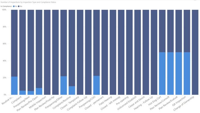
After extensive analysis and exploration in Power BI, some patterns emerge. Quarter 3 is the busiest for inspections, and Quarter 1 is the slowest. Routine inspections occur primarily on Tuesday, Wednesday, or Thursday. Hot dog carts are a roll of the dice.

Inspections by Quarter

Routine inspections by weekday

Inspections by Type

This doesn’t seem too complex, and we theorize that we can create a classifier that predicts whether a restaurant is in compliance, by taking into account the number of violations in each of three categories (priority, core, and foundation).

To do so, we throw together some simple code that ingests the data, splits into a test and training set, creates the classifier model, and provides us the confusion matrix.

# Import the restaurant inspection dataset
df.rst.insp <- read.csv("Restaurant_Inspections_-_All_Inspections.csv", header = TRUE)

# A count of rows in the dataset
num.rows <- nrow(df.rst.insp)

# Create a shuffled subset of rows
subset.sample <- sample(num.rows, floor(num.rows*.75))

# Create a training dataset using a shuffled subset of rows
df.training <- df.rst.insp[subset.sample,]

# Create a test dataset of all rows NOT in the training dataset
df.test <- df.rst.insp[-subset.sample,]

# Create the generalized linear model using the training data frame
mdlCompliance <- glm(In.Compliance ~ Core.Violations + Priority.Violations + Foundation.Violations, family = binomial, data = df.training)

# Predict the compliance of the test dataset
results <- predict(mdlCompliance, newdata=df.test, type = "response")

# Turn the response predictions into a binary yes or no
results <- ifelse(results < 0.5, "No", "Yes")

# Add the results as a new column to the data frame with the actual results
df.test$results <- results

# Output the confusion matrix
table(df.test$In.Compliance, df.test$results)

# Output the confusion matrix
library(caret)
confMat <- table(df.test$In.Compliance, df.test$results)
confusionMatrix(confMat, positive = "Yes")

An accuracy rate of 81.5%! That’s pretty great! Admittedly, a human wouldn’t have much trouble seeing a slew of priority violations and predicting a restaurant shutdown, but this classifier can perform the analysis at a much faster rate.

At this point, we have a good model we trust and expect to use for many years. Let’s pretend to fast forward a decade. Detroit’s meteoric rise has continued, the dataset has grown to massive amounts, and we begin to think we could improve the runtime. Easy enough! Profvis is here to give us the most user-friendly introduction to profiling available. To begin, simply install and load the package.

install.packages("profvis")
library("profvis")

Wrap your code in a profvis call, placing all code inside of braces. The braces are important, and be sure to put every line you want to profile. Maybe your confusion matrix is the bad part, or maybe you read the CSV in an inefficient way!

profvis({

df.rst.insp <- read.csv("Restaurant_Inspections_-_All_Inspections.csv", header = TRUE)
num.rows <- nrow(df.rst.insp)
subset.sample <- sample(num.rows, floor(num.rows*.75))
df.training <- df.rst.insp[subset.sample,]
df.test <- df.rst.insp[-subset.sample,]
mdlCompliance <- glm(In.Compliance ~ Core.Violations + Priority.Violations + Foundation.Violations, family = binomial, data = df.training)
results <- predict(mdlCompliance, newdata=df.test, type = "response")
results <- ifelse(results < 0.5, "No", "Yes")
df.test$results <- results
confMat <- table(df.test$In.Compliance, df.test$results)
confusionMatrix(confMat, positive = "Yes")

})

The output can help pinpoint poor-performing sections, and you can appropriately improve code where necessary.

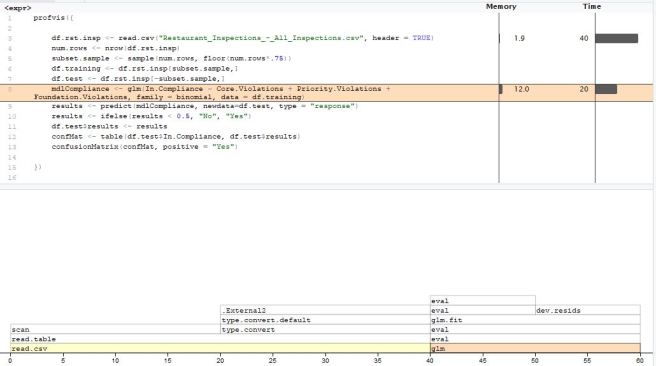
The FlameGraph tab gives us a high-info breakdown. The Data tab gives us the bare-bones stats we need to get started.

profvis FlameGraph

profvis Data tab

In this example, we would certainly choose to improve the way we read in the data, since it accounts for two-thirds of the total run time in that single step!

The result here might be a minor gain, but we can easily understand how larger datasets would see massive performance improvements with a series of tweaks.


Query Azure Cosmos DB in R

It’s 2019, and your company has chosen to store data in Cosmos DB, the world’s most versatile and powerful database format, because they’re all-in on cloud native architectures. You’re excited! This means you’re working with an ultra low latency, planet-scale data source!

Just one problem: your codebase is R, and connecting to retrieve the data is trickier than you’d hoped.

I give you cosmosR: a simple package I wrote to give you a head start on connections to your Cosmos DB. It won’t solve all your problems, but it’ll help you overcome the authentication headers, create some simple queries, and get you up in running much faster than rolling your own connectivity from scratch.

*Note: this is only for Cosmos DB storing documents, with retrieval via the SQL API. For more information on the SQL API please visit the Microsoft documentation.

Begin by making sure we have devtools installed, then loaded:

install.packages("devtools")
library("devtools")

With that set, install cosmosR via GitHub:

install_github("aaron2012r2/cosmosR")

We’re two lines of code away from your first data frame! Be sure to have your Access KeyURIDatabase Name, and Collection Name for your Cosmos DB handy.

Store the access key for reusable querying via cosmosAuth:

cosmosAuth("KeyGoesHere", "uri", "dbName", "collName")

Then we can use cosmosQuery to perform a simple “SELECT * from c” query, which will retrieve all documents from the Cosmos DB. By setting content.response to TRUE, we are specifying that we want to convert the raw response to a character response that we can read.

dfAllDocuments <- cosmosQuery(content.response = TRUE)

Just like that, we have our information! Because documents are stored as JSON, being that Cosmos DB is primarily controlled using Javascript, you should carefully inspect all responses.


The package used in this tutorial is available at my GitHub. Repo linked here. Please visit the link for further information on other tips or known limitations. If you see opportunities to contribute, please branch, create issues, and help further develop!